Microsoft 77-427 Exam Practice Questions (P. 1)
- Full Access (12 questions)
- One Year of Premium Access
- Access to one million comments
- Seamless ChatGPT Integration
- Ability to download PDF files
- Anki Flashcard files for revision
- No Captcha & No AdSense
- Advanced Exam Configuration
Question #1
Change the numbering formats for cell ranges.
* Cell range I7:J7
Accounting -
5 decimal places
$ English (United States)
* Cell range I8:J8
Accounting -
5 decimal places
Japanese
* Cell range I7:J7
Accounting -
5 decimal places
$ English (United States)
* Cell range I8:J8
Accounting -
5 decimal places
Japanese
Correct Answer:
Use the following steps in explanation.
Step 1: Click cell I7, Shift-click cell J7, right-click in this area, and from the context menu select Format Cells.
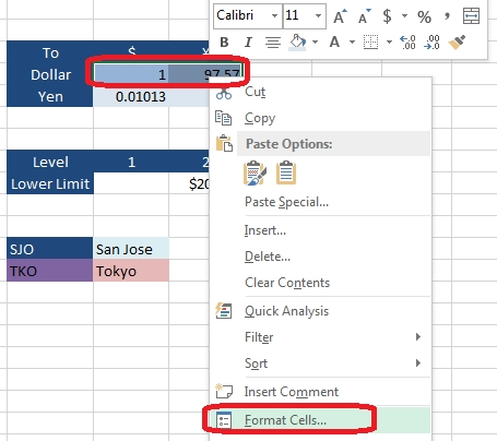
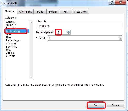
Step 2: In the Format Cells dialog box select Category Accounting, change Decimal places to: 5, and click OK.
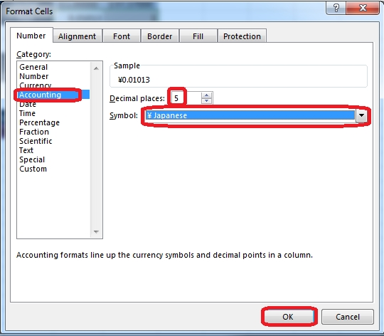
Step 3: Click cell I8, shift-click cell J8, right-click in this area, and from the context menu select Format Cells.
Step 4: In the Format Cells dialog box select Category Accounting, change Decimal places to: 5, set Symbol to: Japanese, and click OK.
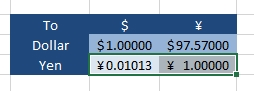
Result will be like:
Use the following steps in explanation.
Step 1: Click cell I7, Shift-click cell J7, right-click in this area, and from the context menu select Format Cells.
Step 2: In the Format Cells dialog box select Category Accounting, change Decimal places to: 5, and click OK.
Step 3: Click cell I8, shift-click cell J8, right-click in this area, and from the context menu select Format Cells.
Step 4: In the Format Cells dialog box select Category Accounting, change Decimal places to: 5, set Symbol to: Japanese, and click OK.
Result will be like:
Question #2
Conditional Formatting.
Use a formula to determine formatting of a cell.
Cell I3 -
Apply formatting if cell is more than three days prior to current date
Use Function TODAY()
Format with Custom solid fill color (RGB R:255 G:59 B:59)
Use a formula to determine formatting of a cell.
Cell I3 -
Apply formatting if cell is more than three days prior to current date
Use Function TODAY()
Format with Custom solid fill color (RGB R:255 G:59 B:59)
Correct Answer:
Use the following steps in explanation.
Step 1: Click cell I3.
Step 2: In the Home tab, click Conditional Formatting, and select New Rule.
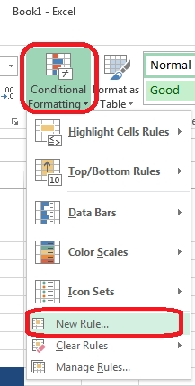
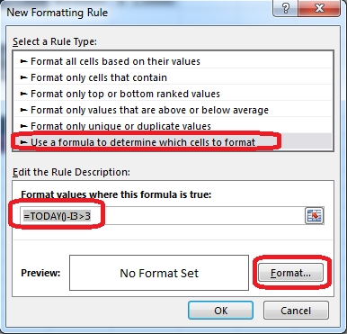
Step 3: In the New Formatting Rule dialog box select Use a formula to determine which cells to format, in the Formal Values where this formula is true type:
=TODAY()-I3>3, and then click the Format button.
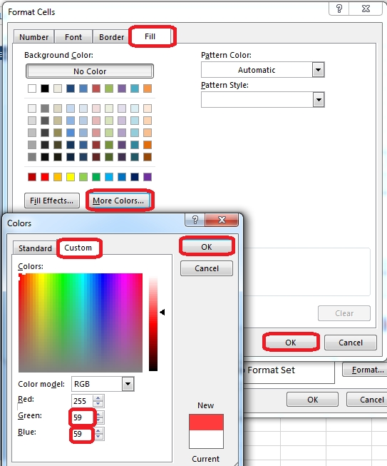
Step 4: In the Format Cells dialog box click the Fill tab, click More Colors, in the Colors Dialog box click the Custom tab, change Green to 59, change Blue to 59, click OK, click OK, and finally click OK in the New Formatting Rule dialog box.
Use the following steps in explanation.
Step 1: Click cell I3.
Step 2: In the Home tab, click Conditional Formatting, and select New Rule.
Step 3: In the New Formatting Rule dialog box select Use a formula to determine which cells to format, in the Formal Values where this formula is true type:
=TODAY()-I3>3, and then click the Format button.
Step 4: In the Format Cells dialog box click the Fill tab, click More Colors, in the Colors Dialog box click the Custom tab, change Green to 59, change Blue to 59, click OK, click OK, and finally click OK in the New Formatting Rule dialog box.
Question #3
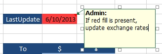
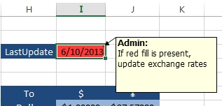
Insert a comment in a cell.
Cell I3 -
Comment text "If red fill is present, update exchange rates"
Cell I3 -
Comment text "If red fill is present, update exchange rates"
Correct Answer:
Use the following steps in explanation.
Step 1: Right-Click in cell I3, and select Insert comment from the context menu.
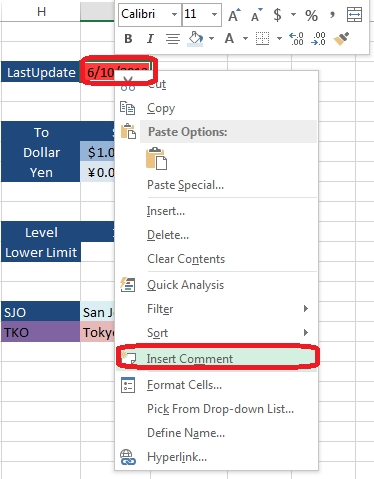
Step 2: Type: If red fill is present, update exchange rates
Step 3: Click cell I3.
You can test by hover above cell I3:
Use the following steps in explanation.
Step 1: Right-Click in cell I3, and select Insert comment from the context menu.
Step 2: Type: If red fill is present, update exchange rates
Step 3: Click cell I3.
You can test by hover above cell I3:
Question #4
Use a function to insert a value in a cell.
Cell range E2:E44 -
The "Level" of each employee -
Function LOOKUP (vector form)
Lookup_value: "$/Hour" (Column D)
Lookup_Vector: Lower Limit row from table.
Cell range E2:E44 -
The "Level" of each employee -
Function LOOKUP (vector form)
Lookup_value: "$/Hour" (Column D)
Lookup_Vector: Lower Limit row from table.
Correct Answer:
Use the following steps in explanation.
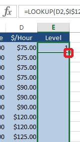
Step 1: Click cell E2, and click the Insert Function button.
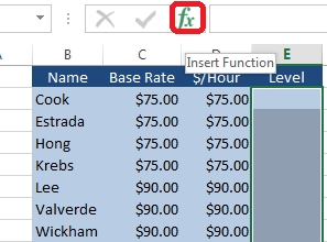
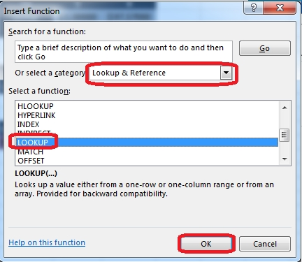
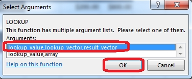
Step 2: In the Insert Function dialog box select Category Lookup & Reference, select function LOOKUP, and click the OK button.
Step 3: In the Select Arguments dialog box make sure lookup, value, lookup vector, result vector is select and click OK.
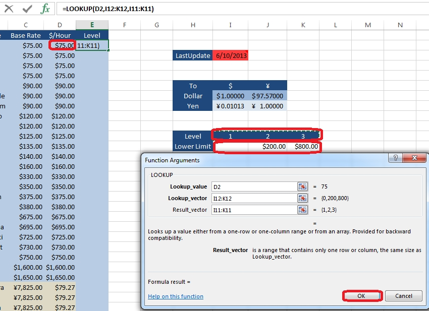
Step 4: For Lookup_value click cell D2, for Lookup_vector select cells I12:K12, for Result vector cells I11:K11, and click the OK button.
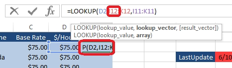
Step 5: Click cell E2, click in cell reference I12 in the formula field, and press the F4 key (to make I12 an absolute reference.
Step 6: Make K12, I11 and K11 absolute references using F4 in the same way.
Result will be:
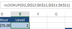
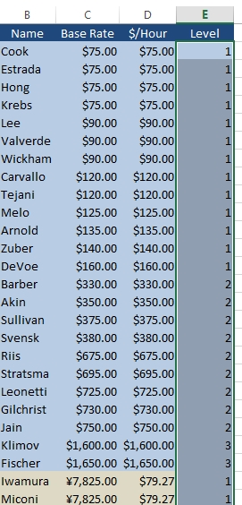
Step 7: Click cell E2, and copy downwards to E44.
Result will be like:
Use the following steps in explanation.
Step 1: Click cell E2, and click the Insert Function button.
Step 2: In the Insert Function dialog box select Category Lookup & Reference, select function LOOKUP, and click the OK button.
Step 3: In the Select Arguments dialog box make sure lookup, value, lookup vector, result vector is select and click OK.
Step 4: For Lookup_value click cell D2, for Lookup_vector select cells I12:K12, for Result vector cells I11:K11, and click the OK button.
Step 5: Click cell E2, click in cell reference I12 in the formula field, and press the F4 key (to make I12 an absolute reference.
Step 6: Make K12, I11 and K11 absolute references using F4 in the same way.
Result will be:
Step 7: Click cell E2, and copy downwards to E44.
Result will be like:
All Pages